Flexibility of the dimensionality reduction assessment
Source:vignettes/dim_reduction_flexibility.Rmd
dim_reduction_flexibility.Rmd## Loading required package: SeuratObject## Loading required package: sp##
## Attaching package: 'SeuratObject'## The following object is masked from 'package:base':
##
## intersect## ── Installed datasets ──────────────────────────────── SeuratData v0.2.2.9001 ──## ✔ pbmc3k 3.1.4 ✔ pbmcMultiome 0.1.4## ────────────────────────────────────── Key ─────────────────────────────────────## ✔ Dataset loaded successfully
## ❯ Dataset built with a newer version of Seurat than installed
## ❓ Unknown version of Seurat installed
library(ClustAssess)
library(ggplot2)
library(harmony)
## Loading required package: Rcpp
library(data.table)

n_repetitions <- 30
The matrix processing parameter of the
assess_feature_stability function is a function that
enables the user to specify any method to perform the dimensionality
reduction prior to applying the UMAP algorithm and the clustering
pipeline. By default, the dimensionality reduction used in
ClustAssess is a precise PCA using the prcomp
package. However, this function can be easily changed, as it will be
shown in the following examples.
ClustAssess using PCA
For the PCA example, we will use the PBMC 3k dataset from the
SeuratData package. The preprocessing of the dataset is
identical with the one performed in the stability pipeline vignette.
InstallData("pbmc3k")## Warning: The following packages are already installed and will not be
## reinstalled: pbmc3k
data("pbmc3k")
pbmc3k <- UpdateSeuratObject(pbmc3k)
## Validating object structure## Updating object slots## Ensuring keys are in the proper structure## Warning: Assay RNA changing from Assay to Assay## Ensuring keys are in the proper structure## Ensuring feature names don't have underscores or pipes## Updating slots in RNA## Validating object structure for Assay 'RNA'## Object representation is consistent with the most current Seurat version
pbmc3k <- PercentageFeatureSet(pbmc3k, pattern = "^MT-", col.name = "percent.mito")
pbmc3k <- PercentageFeatureSet(pbmc3k, pattern = "^RP[SL][[:digit:]]", col.name = "percent.rp")
# remove MT and RP genes
all.index <- seq_len(nrow(pbmc3k))
MT.index <- grep(pattern = "^MT-", x = rownames(pbmc3k), value = FALSE)
RP.index <- grep(pattern = "^RP[SL][[:digit:]]", x = rownames(pbmc3k), value = FALSE)
pbmc3k <- pbmc3k[!((all.index %in% MT.index) | (all.index %in% RP.index)), ]
pbmc3k <- subset(pbmc3k, nFeature_RNA < 2000 & nCount_RNA < 2500 & percent.mito < 7 & percent.rp > 7)
pbmc3k <- NormalizeData(pbmc3k, verbose = FALSE)
pbmc3k <- FindVariableFeatures(pbmc3k, selection.method = "vst", nfeatures = 3000, verbose = FALSE)

features <- dimnames(pbmc3k@assays$RNA)[[1]]
var_features <- pbmc3k@assays[["RNA"]]@var.features
n_abundant <- 3000
most_abundant_genes <- rownames(pbmc3k@assays$RNA)[order(Matrix::rowSums(pbmc3k@assays$RNA),
    decreasing = TRUE
)]

pbmc3k <- ScaleData(pbmc3k, features = features, verbose = FALSE)
We notice that the seurat_annotations column has some
missing values. For simplicity, we will replace them with “NA”.
mask <- is.na(pbmc3k$seurat_annotations)
pbmc3k$seurat_annotations <- as.character(pbmc3k$seurat_annotations)
pbmc3k$seurat_annotations[mask] <- "NA"
Select the features used for the stability assessment.
features <- dimnames(pbmc3k@assays$RNA)[[1]]
var_features <- pbmc3k@assays[["RNA"]]@var.features
n_abundant <- 3000
most_abundant_genes <- rownames(pbmc3k@assays$RNA)[order(Matrix::rowSums(pbmc3k@assays$RNA),
    decreasing = TRUE
)]

steps <- seq(from = 500, to = 3000, by = 500)
ma_hv_genes_intersection_sets <- sapply(steps, function(x) intersect(most_abundant_genes[1:x], var_features[1:x]))
ma_hv_genes_intersection <- Reduce(union, ma_hv_genes_intersection_sets)
ma_hv_steps <- sapply(ma_hv_genes_intersection_sets, length)
Assess the stability of the dimensionality reduction when PCA is used as dimensionality reduction.
matrix_processing_function <- function(dt_mtx, actual_npcs = 30) {
    actual_npcs <- min(actual_npcs, ncol(dt_mtx) %/% 2)

    RhpcBLASctl::blas_set_num_threads(foreach::getDoParWorkers())
    embedding <- stats::prcomp(x = dt_mtx, rank. = actual_npcs)$x

    RhpcBLASctl::blas_set_num_threads(1)
    rownames(embedding) <- rownames(dt_mtx)
    colnames(embedding) <- paste0("PC_", seq_len(actual_npcs))

    return(embedding)
}

pca_feature_stability <- assess_feature_stability(
    data_matrix = pbmc3k@assays[["RNA"]]@scale.data,
    feature_set = most_abundant_genes,
    resolution = seq(from = 0.1, to = 1, by = 0.1),
    steps = steps,
    n_repetitions = n_repetitions,
    feature_type = "MA",
    graph_reduction_type = "PCA",
    matrix_processing = matrix_processing_function,
    umap_arguments = list(
        min_dist = 0.3,
        n_neighbors = 30,
        metric = "cosine"
    ),
    ecs_thresh = 1,
    clustering_algorithm = 1
)
## Warning: executing %dopar% sequentially: no parallel backend registeredPlot the distribution of the celltypes on the UMAP embedding obtained on the top 1000 Most Abundant genes.
umap_df <- data.frame(pca_feature_stability$embedding_list$MA$"1000")
umap_df$celltypes <- pbmc3k$seurat_annotations
ggplot(umap_df, aes(x = UMAP_1, y = UMAP_2, color = celltypes)) +
    geom_point() +
    theme_classic()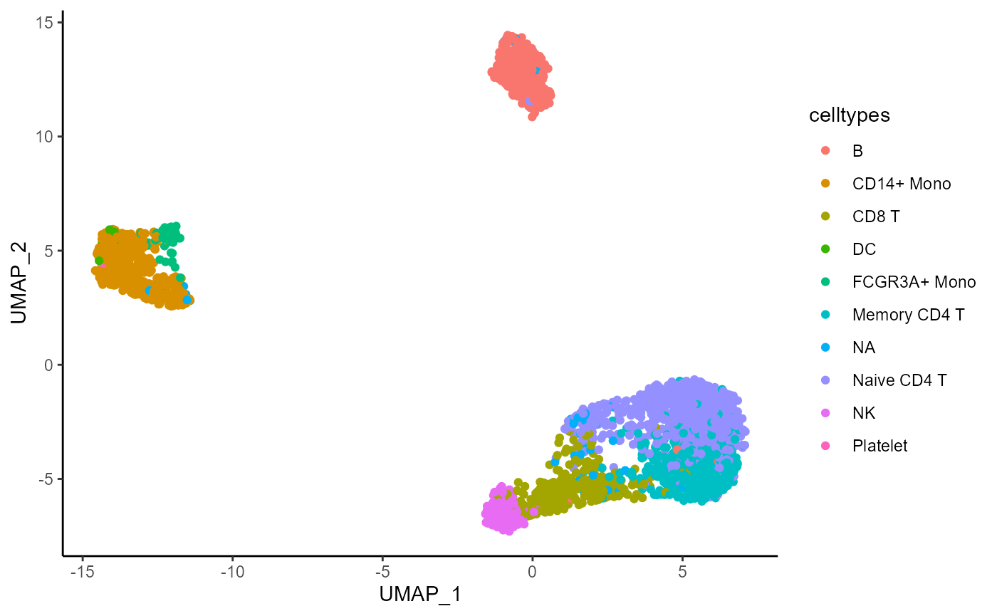
ClustAssess using Harmony
We can also modify the function by adding an addition post-processing step to the PCA. In this example, we will use the Harmony correction to remove the “batch effect” created by the celltypes. Note: This example is meant to exemplify how to use the Harmony correction in the ClusAssess pipeline. The batch correction is actually not needed in the PBMC 3k dataset.
matrix_processing_function <- function(dt_mtx, actual_npcs = 30) {
    actual_npcs <- min(actual_npcs, ncol(dt_mtx) %/% 2)

    RhpcBLASctl::blas_set_num_threads(foreach::getDoParWorkers())
    embedding <- stats::prcomp(x = dt_mtx, rank. = actual_npcs)$x

    RhpcBLASctl::blas_set_num_threads(1)
    rownames(embedding) <- rownames(dt_mtx)
    colnames(embedding) <- paste0("PC_", seq_len(actual_npcs))

    embedding <- RunHarmony(embedding, pbmc3k$seurat_annotations, verbose = FALSE)

    return(embedding)
}

pca_harmony_feature_stability <- assess_feature_stability(
    data_matrix = pbmc3k@assays[["RNA"]]@scale.data,
    feature_set = most_abundant_genes,
    resolution = seq(from = 0.1, to = 1, by = 0.1),
    steps = steps,
    n_repetitions = n_repetitions,
    feature_type = "MA",
    graph_reduction_type = "PCA",
    matrix_processing = matrix_processing_function,
    umap_arguments = list(
        min_dist = 0.3,
        n_neighbors = 30,
        metric = "cosine"
    ),
    ecs_thresh = 1,
    clustering_algorithm = 1,
    verbose = TRUE
)
Plot the distribution of the celltypes on the UMAP embedding obtained on the top 1000 Most Abundant genes.
umap_df <- data.frame(pca_harmony_feature_stability$embedding_list$MA$"1000")
umap_df$celltypes <- pbmc3k$seurat_annotations
ggplot(umap_df, aes(x = UMAP_1, y = UMAP_2, color = celltypes)) +
    geom_point() +
    theme_classic()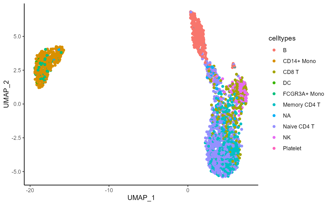
ClusAssess in the ATAC-seq data
In this example we will showcase the flexibility of the
assess_feature_stability function by using the ATAC-seq
data. For this example, we will use the multiome PBMC dataset from the
SeuratData package.
library(Signac)
InstallData("pbmcMultiome")
## Warning: The following packages are already installed and will not be
## reinstalled: pbmcMultiome
data("pbmc.atac")As presented in the (Signac)(https://stuartlab.org/signac/articles/pbmc_vignette) package, the ATAC-seq data is usually processed using the TF-IDF normalization followed by the the calculation of the singular values. These two steps are also known as LSI (Latent Semantic Indexing).
pbmc.atac <- RunTFIDF(pbmc.atac)## Performing TF-IDF normalization## Warning in RunTFIDF.default(object = GetAssayData(object = object, slot =
## "counts"), : Some features contain 0 total countsIdentify the highly variable peaks.
pbmc.atac <- FindTopFeatures(pbmc.atac, min.cutoff = "q5")
var_peaks <- pbmc.atac@assays$ATAC@var.features[seq_len(3000)]
To speedup the assessment, set a parallel backend with 6 cores.
RhpcBLASctl::blas_set_num_threads(1)
ncores <- 6
if (ncores > 1) {
    my_cluster <- parallel::makeCluster(
        ncores,
        type = "PSOCK"
    )

    doParallel::registerDoParallel(cl = my_cluster)
}
Assess the stability of the dimensionality reduction by varying the number of highly variable peaks.
matrix_processing_function <- function(dt_mtx, actual_n_singular_values = 50) {
    actual_n_singular_values <- min(actual_n_singular_values, ncol(dt_mtx) %/% 2)

    RhpcBLASctl::blas_set_num_threads(foreach::getDoParWorkers())
    embedding <- RunSVD(Matrix::t(dt_mtx), n = actual_n_singular_values, verbose = FALSE)@cell.embeddings
    # remove the first component, as it does contain noise - see the Signac vignette
    embedding <- embedding[, 2:actual_n_singular_values]

    RhpcBLASctl::blas_set_num_threads(1)
    rownames(embedding) <- rownames(dt_mtx)
    colnames(embedding) <- paste0("LSI_", seq_len(actual_n_singular_values - 1))

    return(embedding)
}

lsi_atac_feature_stability <- assess_feature_stability(
    data_matrix = pbmc.atac@assays[["ATAC"]]@data,
    feature_set = var_peaks,
    resolution = seq(from = 0.1, to = 1, by = 0.1),
    steps = steps,
    n_repetitions = n_repetitions,
    feature_type = "HV_peaks",
    graph_reduction_type = "PCA",
    matrix_processing = matrix_processing_function,
    umap_arguments = list(
        min_dist = 0.3,
        n_neighbors = 30,
        metric = "cosine"
    ),
    ecs_thresh = 1,
    clustering_algorithm = 1,
    verbose = TRUE
)
## Warning: No assay specified, setting assay as RNA by default.
## No assay specified, setting assay as RNA by default.
## No assay specified, setting assay as RNA by default.
## No assay specified, setting assay as RNA by default.
## No assay specified, setting assay as RNA by default.
## No assay specified, setting assay as RNA by default.
foreach::registerDoSEQ()Plot the distribution of the celltypes on the UMAP embedding obtained on the top 1000 Highly Variable peaks.
umap_df <- data.frame(lsi_atac_feature_stability$embedding_list$HV_peaks$"1000")
umap_df$celltypes <- pbmc.atac$seurat_annotations
ggplot(umap_df, aes(x = UMAP_1, y = UMAP_2, color = celltypes)) +
    geom_point() +
    theme_classic()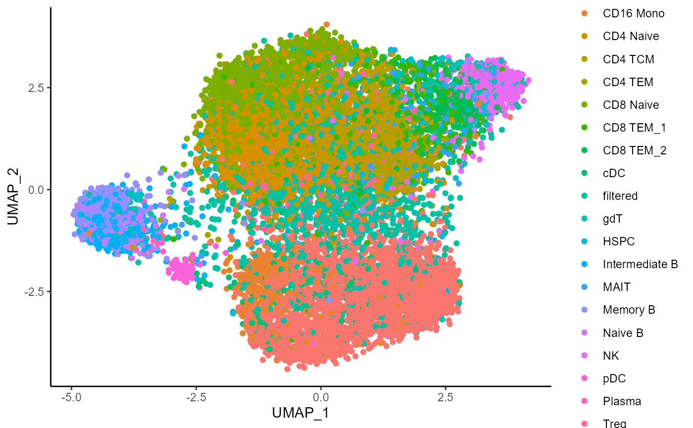
Session info
## R version 4.3.3 (2024-02-29 ucrt)
## Platform: x86_64-w64-mingw32/x64 (64-bit)
## Running under: Windows 11 x64 (build 22631)
##
## Matrix products: default
##
##
## locale:
## [1] LC_COLLATE=Romanian_Romania.utf8  LC_CTYPE=Romanian_Romania.utf8
## [3] LC_MONETARY=Romanian_Romania.utf8 LC_NUMERIC=C
## [5] LC_TIME=Romanian_Romania.utf8
##
## time zone: Europe/Bucharest
## tzcode source: internal
##
## attached base packages:
## [1] stats     graphics  grDevices utils     datasets  methods   base
##
## other attached packages:
##  [1] Signac_1.13.0                 data.table_1.15.4
##  [3] harmony_1.2.0                 Rcpp_1.0.12
##  [5] ggplot2_3.5.0                 ClustAssess_1.0.0
##  [7] pbmcMultiome.SeuratData_0.1.4 pbmc3k.SeuratData_3.1.4
##  [9] SeuratData_0.2.2.9001         Seurat_5.0.3
## [11] SeuratObject_5.0.1            sp_2.1-3
##
## loaded via a namespace (and not attached):
##   [1] RcppAnnoy_0.0.22        splines_4.3.3           later_1.3.2
##   [4] bitops_1.0-7            tibble_3.2.1            polyclip_1.10-6
##   [7] fastDummies_1.7.3       lifecycle_1.0.4         doParallel_1.0.17
##  [10] globals_0.16.3          lattice_0.22-5          MASS_7.3-60.0.1
##  [13] magrittr_2.0.3          plotly_4.10.4           sass_0.4.9
##  [16] rmarkdown_2.26          jquerylib_0.1.4         yaml_2.3.8
##  [19] httpuv_1.6.15           sctransform_0.4.1       spam_2.10-0
##  [22] spatstat.sparse_3.0-3   reticulate_1.35.0       cowplot_1.1.3
##  [25] pbapply_1.7-2           RColorBrewer_1.1-3      abind_1.4-5
##  [28] zlibbioc_1.48.2         Rtsne_0.17              GenomicRanges_1.54.1
##  [31] purrr_1.0.2             BiocGenerics_0.48.1     RCurl_1.98-1.14
##  [34] rappdirs_0.3.3          GenomeInfoDbData_1.2.11 IRanges_2.36.0
##  [37] S4Vectors_0.40.2        ggrepel_0.9.5           irlba_2.3.5.1
##  [40] listenv_0.9.1           spatstat.utils_3.0-4    goftest_1.2-3
##  [43] RSpectra_0.16-1         spatstat.random_3.2-3   fitdistrplus_1.1-11
##  [46] parallelly_1.37.1       pkgdown_2.0.7           leiden_0.4.3.1
##  [49] codetools_0.2-19        RcppRoll_0.3.0          tidyselect_1.2.1
##  [52] farver_2.1.1            matrixStats_1.2.0       stats4_4.3.3
##  [55] spatstat.explore_3.2-7  jsonlite_1.8.8          progressr_0.14.0
##  [58] ggridges_0.5.6          survival_3.5-8          iterators_1.0.14
##  [61] systemfonts_1.0.6       foreach_1.5.2           tools_4.3.3
##  [64] progress_1.2.3          ragg_1.3.0              ica_1.0-3
##  [67] glue_1.7.0              gridExtra_2.3           xfun_0.43
##  [70] GenomeInfoDb_1.38.8     dplyr_1.1.4             withr_3.0.0
##  [73] fastmap_1.1.1           fansi_1.0.6             digest_0.6.35
##  [76] R6_2.5.1                mime_0.12               textshaping_0.3.7
##  [79] colorspace_2.1-0        scattermore_1.2         tensor_1.5
##  [82] spatstat.data_3.0-4     RhpcBLASctl_0.23-42     utf8_1.2.4
##  [85] tidyr_1.3.1             generics_0.1.3          prettyunits_1.2.0
##  [88] httr_1.4.7              htmlwidgets_1.6.4       uwot_0.1.16.9000
##  [91] pkgconfig_2.0.3         gtable_0.3.4            lmtest_0.9-40
##  [94] XVector_0.42.0          htmltools_0.5.8         dotCall64_1.1-1
##  [97] scales_1.3.0            png_0.1-8               knitr_1.45
## [100] reshape2_1.4.4          nlme_3.1-164            cachem_1.0.8
## [103] zoo_1.8-12              stringr_1.5.1           KernSmooth_2.23-22
## [106] parallel_4.3.3          miniUI_0.1.1.1          desc_1.4.3
## [109] pillar_1.9.0            grid_4.3.3              vctrs_0.6.5
## [112] RANN_2.6.1              promises_1.2.1          xtable_1.8-4
## [115] cluster_2.1.6           evaluate_0.23           cli_3.6.2
## [118] compiler_4.3.3          Rsamtools_2.18.0        rlang_1.1.3
## [121] crayon_1.5.2            future.apply_1.11.2     labeling_0.4.3
## [124] plyr_1.8.9              fs_1.6.3                stringi_1.8.3
## [127] viridisLite_0.4.2       deldir_2.0-4            BiocParallel_1.36.0
## [130] munsell_0.5.1           Biostrings_2.70.3       lazyeval_0.2.2
## [133] spatstat.geom_3.2-9     SharedObject_1.16.0     Matrix_1.6-5
## [136] RcppHNSW_0.6.0          hms_1.1.3               patchwork_1.2.0
## [139] future_1.33.2           shiny_1.8.1.1           highr_0.10
## [142] ROCR_1.0-11             igraph_2.0.3            memoise_2.0.1
## [145] bslib_0.7.0             fastmatch_1.1-4